Excel How To Color Every Other Row
Alright, gather 'round, you magnificent spreadsheet wranglers and data dabblers! Today, we're going to tackle a problem that has plagued humanity for… well, at least since the invention of the spreadsheet. You know the feeling, right? You’ve got a colossal chunk of data, a veritable Everest of numbers and text, and it looks like a herd of caffeinated squirrels threw a party on your screen. It's an absolute visual nightmare. Your eyes are doing this weird, jiggly thing, and you're pretty sure you've accidentally added up your cat's kibble count with your quarterly profit margins. Tragic.
But fear not, my friends! Because there’s a simple, elegant, and dare I say, glorious way to bring order to this chaos. We’re talking about coloring every other row. Yes, I know, it sounds like something out of a wizard's grimoire, but trust me, it’s as easy as… well, as easy as convincing your boss that "strategic napping" is a valid professional development activity.
Now, before we dive in, let’s appreciate the sheer, unadulterated beauty of this technique. It’s like putting little striped pajamas on your data. Suddenly, everything is easier to read, to digest, to understand. It’s the difference between staring at a blurry phone number scribbled on a napkin and reading it off a pristine, laser-printed business card. You’ll be able to spot trends faster than a hawk spotting a particularly plump field mouse. You might even start seeing patterns in your grocery bill that you never knew existed. Maybe you're spending more on cheese than you thought? Shocking, I know.

So, how do we achieve this spreadsheet nirvana? It’s not about clicking and dragging with your mouse until your carpal tunnel starts sending you passive-aggressive emails. Oh no, we’re going to be sophisticated. We're going to leverage the magical power of Conditional Formatting.
The Ancient Art of Making Rows Look Pretty (Without Losing Your Mind)
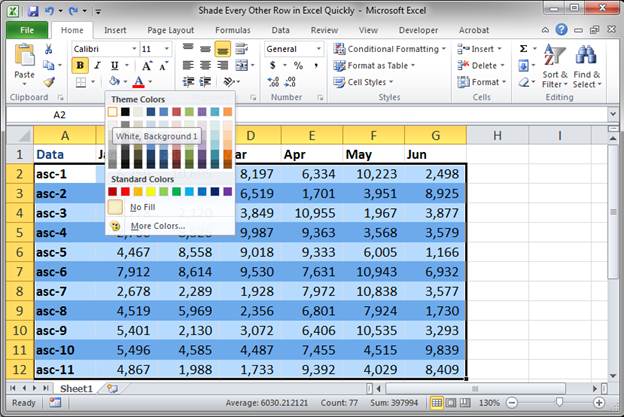
First things first, you need to open your Excel file. Go ahead, I’ll wait. Take a deep breath. Feel the hum of the computer. This is where the magic happens. Now, you need to select the data you want to jazz up. Think of it as selecting your favorite outfit before a big date. You want to make sure it's looking its best. You can click and drag your mouse, or if your data is particularly massive (we're talking "millions of rows" massive, like that one time I tried to catalog every single crumb I'd ever dropped), you can use keyboard shortcuts. Ctrl+A (or Cmd+A on a Mac) will usually select your entire active data set. Boom! Instant selection.
Once your data is highlighted, like a celebrity under a spotlight, it’s time to find our magical tool. Look for the Conditional Formatting option. It’s usually hiding in plain sight on the Home tab, nestled amongst other exciting buttons like "Format Painter" (which is also surprisingly useful, but that’s a story for another latte). Click on it. Don't be shy. It's friendly.
Unleashing the Power of Formulas (Don't Panic!)
Now, a little menu will pop up, looking a bit like a choose-your-own-adventure book. We're going to scroll down, past the "Color Scales" and "Icon Sets" (which are also fun, but we're on a mission today!), until we find New Rule. Click that bad boy.
Here’s where it gets a little… mathematical. But I promise, it's not like trying to solve a Rubik's cube blindfolded. We want to select the option that says "Use a formula to determine which cells to format". Yes, it sounds daunting, but think of it as giving Excel a secret handshake.
In the little box that appears, we're going to type in a formula. This is the secret sauce, the incantation, the… well, it's the formula! Don't worry, I've got you. The formula you need to type is:
=MOD(ROW(),2)=0
Let's break this down, shall we?
- ROW(): This is like asking Excel, "Hey, what row number are we looking at right now?" Excel, being the obedient servant it is, will tell you. So, for the first row, it's 1, for the second, it's 2, and so on.
- MOD(): This is the modulo operator. It’s basically asking for the remainder after division. So, if you divide 5 by 2, the remainder is 1. If you divide 6 by 2, the remainder is 0. Simple, right?
- =0: We’re specifically looking for rows where the remainder is 0 when divided by 2. This means we’re targeting the even-numbered rows. Why even? Because usually, the first row is your header, and you might want to leave that one plain. But hey, you do you! If you want to color every other row starting from the very first, you can use
=MOD(ROW(),2)=1for odd numbers.
So, in plain English, this formula is saying: "If the row number, when divided by 2, has a remainder of 0 (meaning it's an even row), then apply the formatting."
The Grand Finale: Choosing Your Colors!
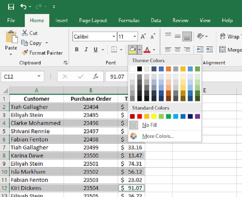
Now that we’ve told Excel which rows to format, we need to tell it how to format them. See that little Format... button? Click it. This is where you unleash your inner interior decorator.
You'll get another window, this one looking like a paint palette. Go to the Fill tab. This is where the magic happens! Choose a color that makes your heart sing. Are you feeling a sophisticated, muted grey? Or perhaps a bold, "I just closed that multi-million dollar deal" kind of teal? The choice is yours!
Once you’ve picked your fabulous hue, click OK. Then, click OK again on the next window. And behold! Your spreadsheet is transformed. Those rows are now alternating in glorious color. You might even feel a sudden urge to high-five yourself. Go ahead, you've earned it.
Why This Little Trick is a Spreadsheet Game-Changer
This isn't just about making your data look pretty (though that's a huge perk!). Properly formatted data is easier to read, which means you'll make fewer mistakes. Think about it: no more accidentally adding your rent payment to your inventory costs. No more confusing your colleague's birthday with a critical project deadline. This is about clarity, efficiency, and, dare I say, a little bit of peace of mind.
It's also a fantastic time-saver. Imagine having to manually color every other row in a thousand-row spreadsheet. You’d be there until the next solar eclipse. With this conditional formatting trick, you can apply it in seconds, and it automatically updates if you add or delete rows. It’s like having a tiny, efficient butler for your data.
So, the next time you’re faced with a data sheet that looks like a Jackson Pollock painting gone wrong, remember this little trick. You'll be the hero of your office, the guru of spreadsheets, the one who brought order to the chaos. And who knows, maybe you’ll even start seeing the world in alternating stripes. Now, if you'll excuse me, I think I need another coffee to process all this excitement. Happy spreadsheeting!